
In astronomy, the processing of spectroscopic data is a relatively repetitive action. When we say repetitive, we mean theoretically automatable. In this article, I propose you to try a quick and code-free approach of this automation.
When you are an amateur astronomer, whether you practice astrophotography or spectroscopy, the data accumulate quickly and in mass. In addition to the need to organize them intelligently to find them, it is often useful to process them shortly after acquisition to remember any particularities and keep the session in mind. Automating these processes saves time so that you can concentrate on analyzing the data.
Rather than providing a software or a turnkey solution, I propose to build together a process that can adapt to your constraints and uses, at least I hope so. This without typing a line of code, while allowing you to add to it as you wish. Indeed, for several years now, a trend has been developing and making a small place in the ways of implementing applications, the No Code trend.
No Code
This practice of No Code aims at assembling pre-programmed and configurable software bricks in order to design software, such as mobile applications or processes, but without having to code, you will have understood. This solution does not meet all needs, however it is sometimes possible to add or execute code in addition. So I propose to use one of these solutions to build our process, in “no code”.
Acquisition
Here, we will assume that the acquisition solution is left to the astronomer’s choice. Besides the advantage of allowing each one to use the acquisition solution that he or she prefers, this will also allow us to keep the automatic reduction process as it is tomorrow if we change the acquisition software.
Several softwares allow to acquire spectra easily such as Prism or MaximDL which also allow to automate the acquisitions by complementary scripts. Here, I used the INDI distributed communication protocol associated with the KStars planetarium, already presented in another article : Spectre de Phecda.
To illustrate our process, let’s start with an observation made with the Star’Ex spectroscope, in 3D printing, implemented by C. Buil (see project page here : https://astrosurf.com/solex/starex).

The core of the reduction process can be done with the SpecINTI software which needs two files :
The file describing the observation and the resulting files.
The file describing the hardware configuration and the processing options to be applied.
We will come back to these files and their configurations a little later.
This executable is accompanied by a folder named _configuration which is placed in the same place where we will place the famous file describing the hardware and the processing. For more information on the software and its operation, I can only advise you to visit the project page of C. Buil which details everything very well, at this address : http://www.astrosurf.com/solex/specinti.html.
This SpecINTI reduction engine exists in different versions that can be run on the most common operating systems. This makes it possible to use this automation solution on Windows, macOS, Linux, and also on Raspberry Pi. What better than a compact, low-power Raspberry Pi board for this ?
Automation with n8n
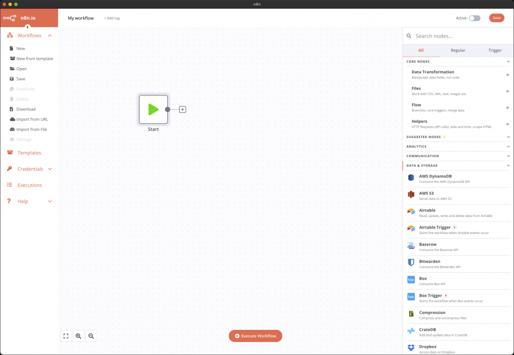
Now that we have everything we need, we can unfold the process that will be applied as soon as a session is to be processed. To implement this process, we will use the tool called n8n (pronounced n – eight – n) which is a node-based workflow automation tool.
Official Website : https://n8n.io/
This tool has a really easy and pleasant interface to use thanks to which we can, by a simple drag and drop, build our different steps.
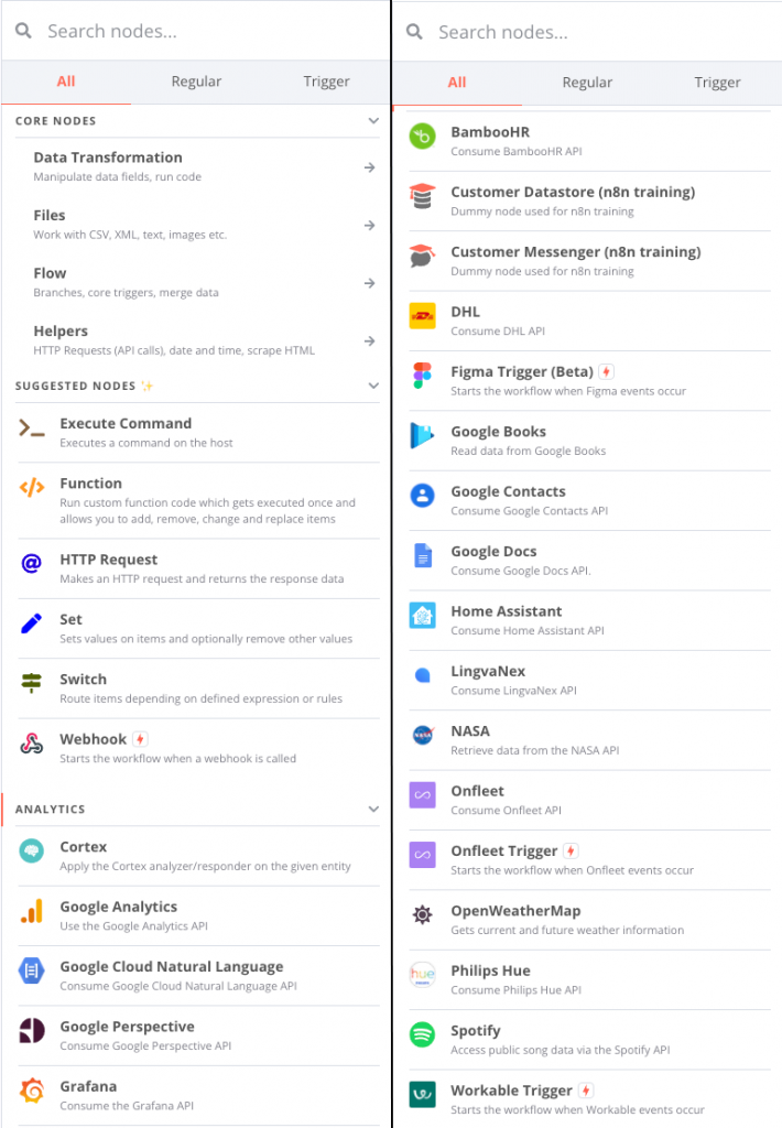
for example, can be configured. Many types of nodes already exist, from simple operations such as reading CSV files, retrieving data from APIs such as NASA’s, but also a host of online services such as Dropbox, Google Drive and so on.
Three installation modes are possible:
| Auto Hébergé | Desktop | Cloud |
| Installation of the solution manually, in other words self-hosted, for example on Raspberry Pi! This mode is free. | Install the application on your personal machine (Windows, macOS, and soon Linux). This mode is free. | Use of the solution in cloud mode, online. This mode is not free. |
So that the steps described here can be reproduced easily and by the greatest number of people, we will use the second solution, namely the office application.
Not much differs between operating systems regarding the use of the application, it’s mostly about different paths or system specific commands. However, in order to cater for the widest range of uses, I have written this same article according to the operating system on which you will be using the application.
Linux, but a PDF version for Windows is available below. It will allow you to follow this article to discover the solution together, but also to test on your machine afterwards.
PDF for macOS version

PDF for Windows version
Moreover, all the observation files used and the process we are going to build can be downloaded at the end of this article. So, let’s go. Go to the official website of n8n, here: https://n8n.io/, select Desktop app at the bottom of the page and follow the standard installation instructions.
First steps on n8n
So now we have our application open, on the desktop. On the left is the workflow management menu with the classic operations, new, open, save, … The center of the window will contain all the graphic steps of our process. When a new process is created, a Start item is displayed. On the right are the famous nodes that we will use, we just have to click on one of the nodes to add it to the central space and connect them together to use them.
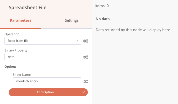
Once added, double-clicking the node allows access to its configuration. For example, the Speadsheet File node allows you to read or write a CSV or XLS file.
I propose that we now outline our automatic reduction flow. To keep it simple, we’ll take the example of an observatory where there is a remotely controlled computer that controls the equipment and contains the files of the last session recorded the day before. We therefore assume that the n8n application is installed on this computer.
On this computer, we also have a working folder in which we have the observation files and everything else we will need for this automation. Here is the global tree structure of this working folder :
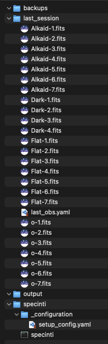
- A backups folder in which we will save our session files before each processing to avoid losing our session if our processing chain goes wrong…
- A last_session folder that contains all our observation files to process
- A specinti folder which contains the SpecINTI executable and the hardware configuration file.
- An output folder
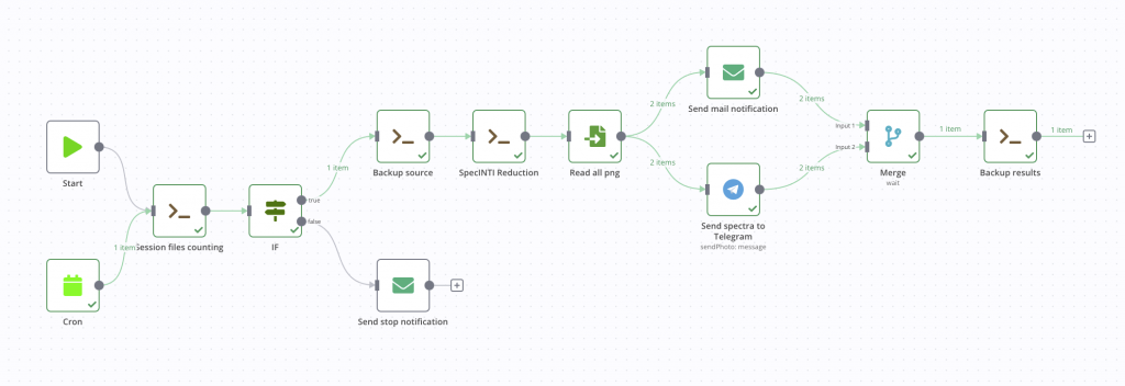
The steps, when triggering our pipeline, will be :
Verification of the presence of files to be processed
⬇️
Backup of files (a copy in another local folder)
⬇️
Launch of the reduction with SpecINTI
⬇️
Envoi d’une notification à l’astronome pour lui préciser la fin de traitement
⬇️
Sending a notification to the astronomer to specify the end of the treatment
We’ll take the time to get started by detailing the first few steps, then add the steps more quickly after that.
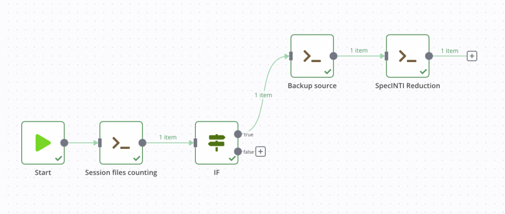
Automatic Reduction Pipeline (Lite)
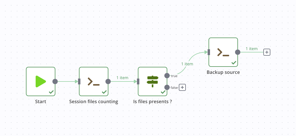
Verification of the presence of the files to be processed
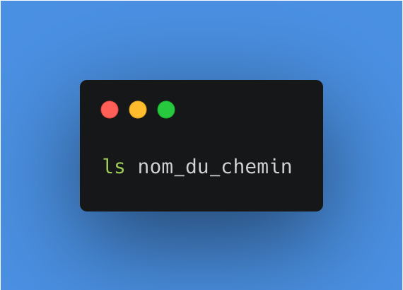
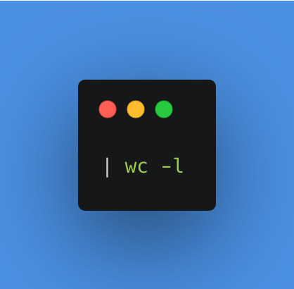
Each time the process is started, we will check if any files are present, if so, the process will stop. To do this, we can use a command to list the files present in a folder and count them. On macOS, this terminal command (bash) is the following:
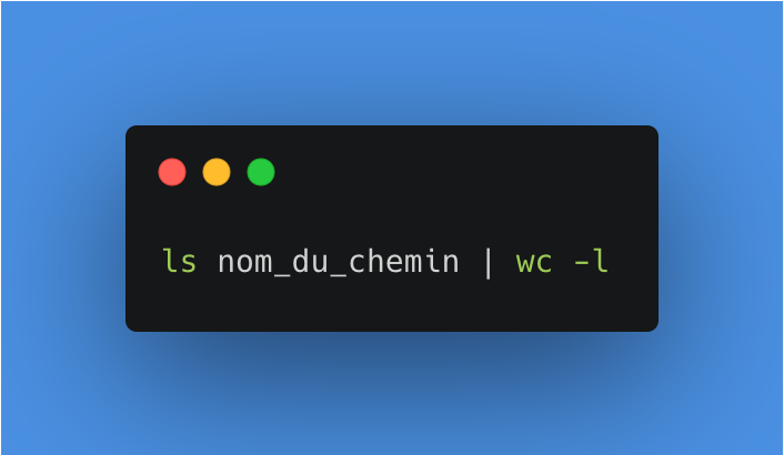
Here are the details, first we list all the files in the last_session folder.
Then we redirect this list of files to another command thanks to the pipe, then we count the number of words/lines/characters with wc. The -l option allows us to specify that we want to count the lines, i.e. all the files present.
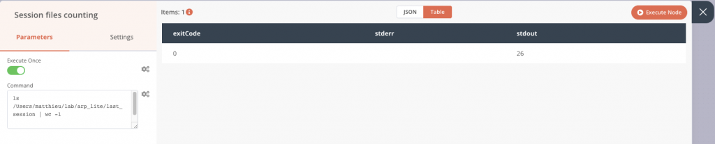
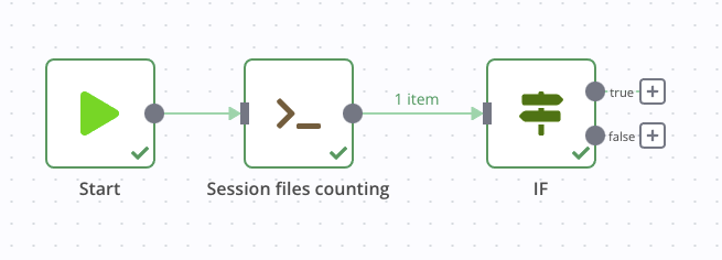
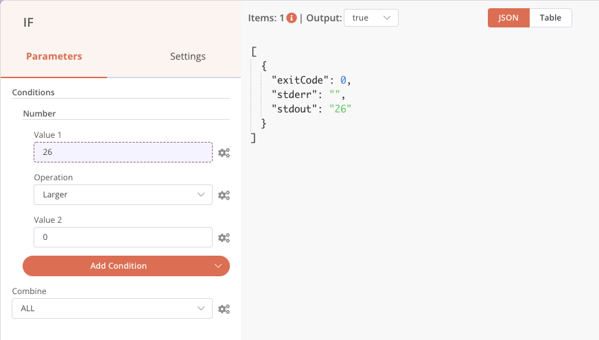
In the application, I add the node called Execute Command, in which I will integrate the previous command. In this configuration, we can already see the output on the right panel during a test execution. Here the package contains 26 files that we find in the stdout column. All is good, I can connect it to the first Start node.
Now we can retrieve this output from a next node and use it as a condition, with the IF block. If files are present, we continue, otherwise we stop. First, let’s connect the if block to the previous node without setting any parameters and run the whole chain. This will allow us to graphically recover the number of files counted previously.
Once that’s done, we can set it up by double-clicking on this IF node, then adding a Number condition. In the first value field, click on the little cogwheel to add an expression, as below:
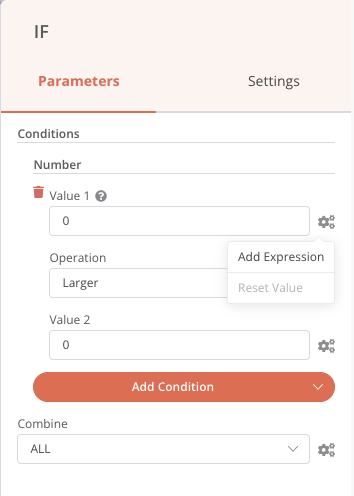
A new window opens, and we can go and get the value of stdout in the inputs. By clicking once, the element is added. If we had not performed the previous execution, the input value would not have been present in the list, because it was not yet known. But it is still possible to add it manually in the right field.
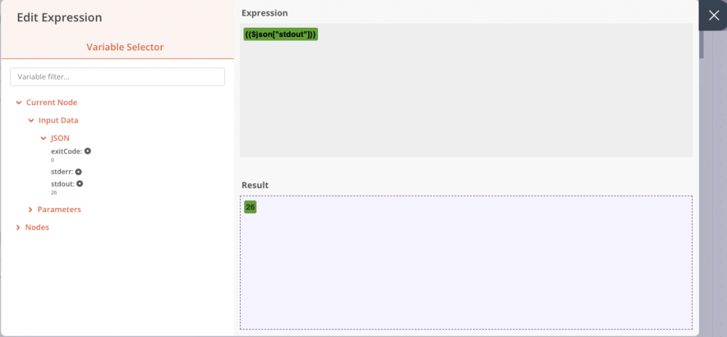
The other condition fields are configured so that if stdout, which we have just retrieved, is greater than 0, then files are present and the output will be True. Note that this is a fairly light check, you could simply have several text files and the condition would be validated. You are of course free to reinforce this check afterwards.
Our file presence verification step is complete.
Backup of files
To save this file folder, again we can use the ease of use of our system commands, by making a simple copy to another folder. But we can also use a Google Drive node, Dropbox, or the FTP node to save our files elsewhere.
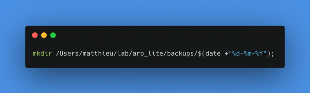
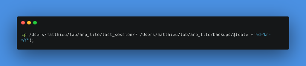
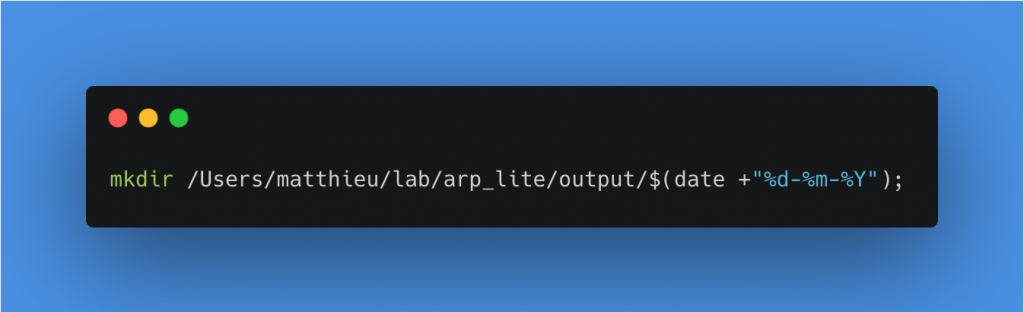
To make this copy, I will create a folder by giving it the name of the processing date inside the Backups folder. To do this, I add the following two commands in a row in the same Execute commands block. Of course, you have to replace the path of the last_session and backup folders with your own.
Create a folder with the current date in backups
Copy all files from the last_session folder to the backups/date-of-day folder
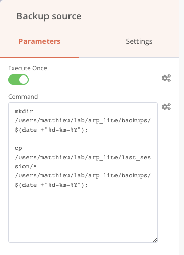
We then connect this node to the True output of our previous If node, this step is complete.
Reduction with SpecInti
We are ready to launch the reduction. SpecINTI is available as executables, which can be launched with a simple system command. It’s a good thing we know the Execute command node well. Don’t worry, we’ll see other nodes right after!
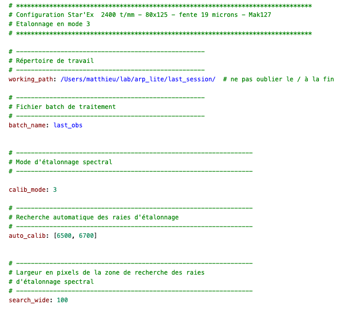
So I downloaded the SpecINTI executable for macOS via this page : SpecINTI MacOS & Linux, and the hardware and processing configuration file in the _configuration folder. Our configuration file should always have the same name, because it will be called at each processing. Here it is called setup_config.yaml
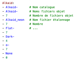
Furthermore, the first two parameters to be specified in this configuration file are the path of the entire observation files. And the name of the observation file which specifies the names of the FITS files. As we are going to automate the processing, it is important that the observation file always has the same name. Here I have chosen to call it last_obs.yaml
We already met a thumbnail of this file at the beginning of this article, I put it back here to illustrate my point.
⚠️ Reminder of the automation rules
| If our hardware does not change, the configuration file theoretically does not change. The configuration file will always be named setup_config.yaml | The files to be processed will always be in the last_session | The observation file will always be named last_obs.yaml |
So let’s add an Execute Command node that calls SpecINTI and performs this reduction.
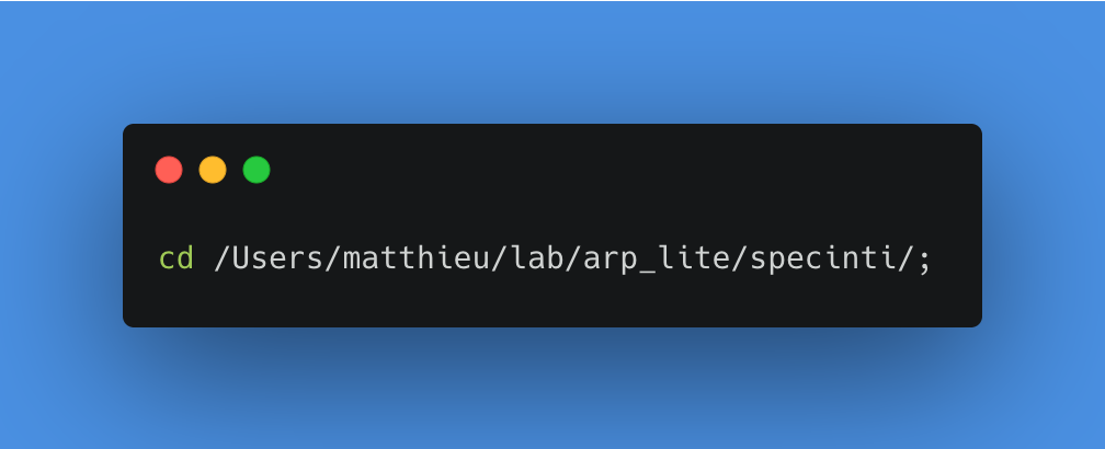
Move to the specinti folder
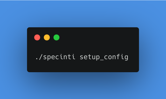
Launching SpecINTI with the configuration file as parameter
And that’s it!
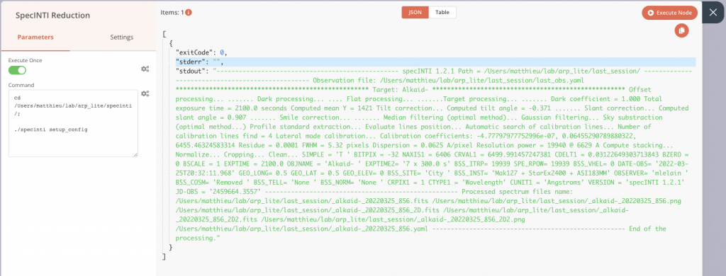
After its execution, or during a test run, we find the classic output of SpecINTI on stdout, with the various information of the treatment which are displayed in the terminal in normal time. Here is what our pipeline looks like at this stage.
Notification of end of treatment
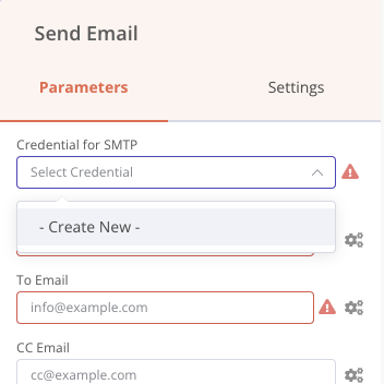
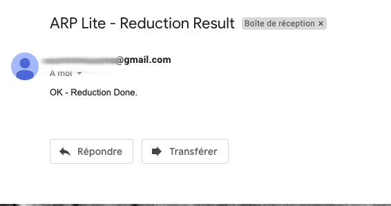
Now that the reduction is complete, we can add a node to warn the astronomer that his data is ready, for example with the node Send email.
The first step is to add an email account to be able to send emails, with the classic login information, email address, password, host server. All the connection information is saved only on your machine and is then accessible in the Credentials menu of the application. Let’s add this node Send Email.
Then we can configure the message we want to send to a destination address.
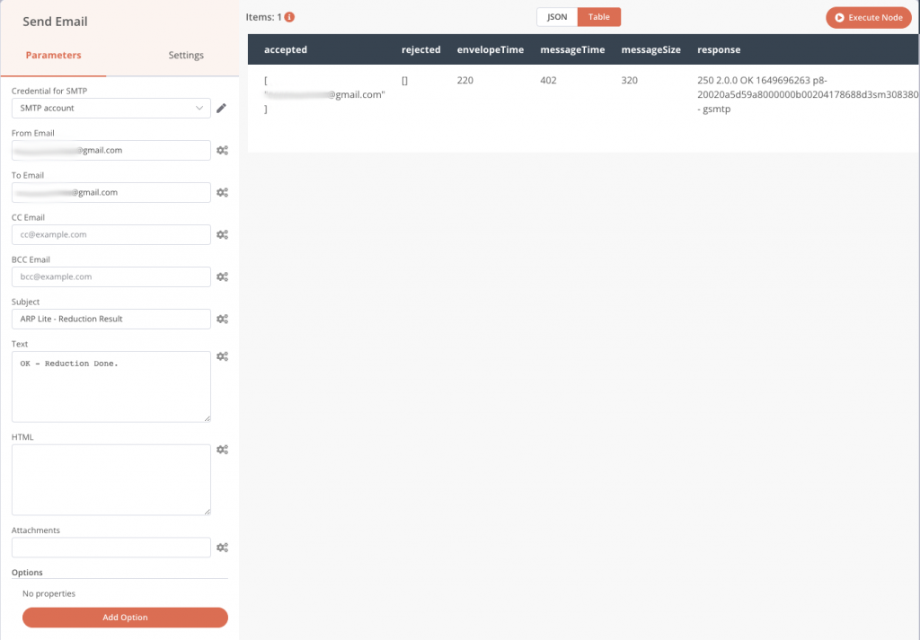
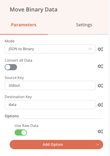
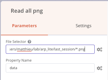
We can also precede the Send email node with a Read Binary Files node that will read all the PNG files in the results folder and send them to the output named data, and then we can embed these images (named data) in the notification email as in the previous screenshot (attachment fields).
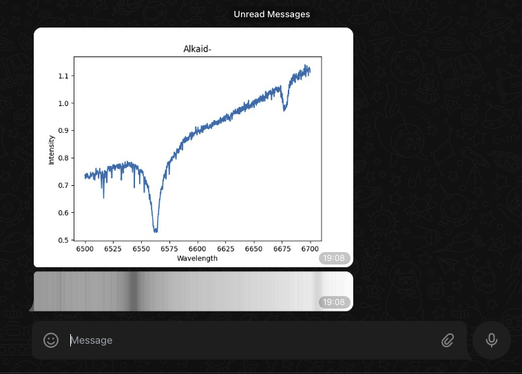
The same logic can be applied with the Telegram node (instant messaging application comparable to WhatsApp) to which we send the list of PNG files received, and thus we receive a message directly in a conversation.
Below is the result of the mobile notification on the right and the status of our process.
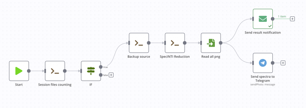
Saving the results
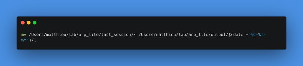
We can now finalize our processing chain with a backup of the results. To make it simple, we will simply move the files to the output, in a new folder named with the current date as for the first backup. This time we will use the move command in an Execute Command node.
It is important to move all the files rather than making a copy, because tomorrow a new session may have to be processed. So we have to empty the last_session folder.
Create a new folder in output with the current date as name
Move all files from the last_session folder to the folder created just before
To do things properly, we can add a Merge node beforehand that will wait for the two notifications to be sent before starting the backup. We can also duplicate the email sending to warn the astronomer if the process stops at the beginning when there are no files to process.
Trigger
Our processing chain is now finalized. However, it is only triggered manually, not very automatic… Let’s add a cron so that it is triggered every day at 2pm precisely.
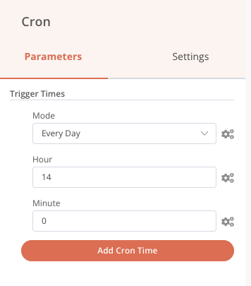
Each day the processing will be done if there are files present, otherwise it will stop. We also always have the possibility to start it manually with the Start node if the 14 h wait is unbearable!
The Local files Trigger node is also a possibility. It can be configured to check for file additions or changes in a folder. Thus, we could very well trigger our processing chain once all acquisitions are completed at the end of the night by simply adding a last FITS image of one second pose with a particular name that will serve as a trigger, session_end.fits for example.
This time it’s good, our automatic processing pipeline is finished! Here is the graphic result.
You will also find below the entire code of this process in JSON format. To use it, nothing could be easier, in the application menu, select Import from file, you’re done. You will still need to modify the nodes with your own machine paths and mail connection information if you want to keep it as is.
I also put the whole folder with the FITS files and the observation and configuration files that will give you everything you need.
macOS


Windows
Extension and opening
This process is an example. The processing chain described here is intended to provide an introduction by giving the keys to starting and running your own process. During automatic processing, it is important to take into account all the situations that may arise according to their probable frequency of occurrence (power failure in the middle of processing, incomplete data, etc.).
The same is true for the solution chosen here. The advantage of this solution, n8n, is to be able to answer to multiple configurations and technical knowledge levels. For example, an advanced user can use the Execute command block (the famous one!) to launch a Python script in which he will have integrated powerful treatments while keeping the graphical simplicity for the management of the global chain. It is not impossible that a new article will be published soon using this possibility.
Other solutions exist depending on the use:
| NodeRed | Airflow |
| The NodeRed solution is a very close alternative to the one used here, also in JavaScript. The documentation is very well done and there are many videos and articles with relevant examples online. | We also note the Airflow solution in Python. This last one is rather intended for Python developers. It requires a more important hardware configuration and a Linux server, or even Docker. That said, it can meet more important needs in terms of processing. It is for example the solution that is implemented for the 2SPOT association (https://2spot.org/FR) which benefits from many clear skies in Chile and thus from a regular and consequent volume of data to be processed. |
| https://nodered.org | https://airflow.apache.org |
Hoping that this article can be useful for your uses, do not hesitate to contact me if you have any questions or if you want to exchange on these solutions of course.
Thanks for reading this far ! 🙂
Sources & References
Header image : https://unsplash.com/photos/Pp9qkEV_xPk